BAS Radiation Belt Model (BAS-RBM)
BAS Radiation Belt Model (BAS-RBM)
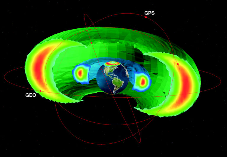
The radiation belts are regions of space around Earth where high-energy charged particles are trapped by our planet’s magnetic field.
Many factors influence the energy of these particles and their distribution in space, including the solar wind, interactions between particles and electromagnetic waves, and activity on the Sun. The relationship between these factors and the charged particle population is complex, making radiation belt dynamics an area of intense international research.
Understanding the processes in the radiation belts matters beyond scientific curiosity. High-energy electrons can damage satellites, disrupt satellite services such as GPS navigation and communications, endanger spacecraft crew, and may even influence our climate by causing chemical reactions in the upper atmosphere.
The BAS-RBM simulates changes in the high-energy electron population of the radiation belts, taking into account effects such as changing solar activity and wave-particle interactions. This helps to improve our understanding of the processes involved and supports the development of warning and forecasting capabilities.
BAS-RBM produces an automated forecast of the radiation belts every hour with a forecast period of 24 hours. The forecasts are available via the European Space Agency web portal.
The forecast are used by satellite operators, insurance underwriters and satellite designers to help ensure the safe and reliable operation of satellite services.
The model has been licensed to the UK Met Office and is being developed into an operational model for the UK.

The Earth’s electron radiation belts
Summary of features for the BAS Global Dynamic Radiation Belt Model
| Type of model | 3 dimensional, time-dependent diffusion model for phase-space density based on solution of the Fokker-Planck equation |
| Diffusion coefficients | Radial diffusion coefficients are taken from [Brautigam & Albert ,JGR,2000] Pitch-angle and energy diffusion coefficients are calculated using the PADIE code [Glauert & Horne, JGR, 2005]. |
| Co-ordinate system | The model uses 2 coordinate systems to construct computational grids: (L*, α, E) and (L*, μ, J) |
| Numerical method | Implicit finite difference scheme |
| Required Inputs | A time-series of Kp for the period in question |
| Optional Inputs | The initial particle flux or phase space density The variation of particle flux or phase space density with time on the boundaries in L* and E |
| Wave-particle interaction models | BAS chorus model BAS hiss model which includes diffusion due to lightning and hiss in plumes These MLT averaged models were derived using the BAS wave database Other wave-particle interactions can also be included |
| Pitch-angle, energy and L-shell ranges | 0o ≤ pitch-angle ≤ 90o The energy and L-shell grids can be varied but typically 1 ≤ L*≤ 7 and 10 MeV/G ≤ μ ≤ 2000 MeV/G at L* = 6.5 |
| Outputs | The model produces a time-series of the flux or phase-space density on the 3-d grid |